Endoluminal Robotics Workflows#
Workflows for navigation and intervention through luminal anatomy.
Workflows#
| Workflow | Demonstration | Supported modes (guide) |
|---|---|---|
endoluminal_navigation |
Navigate a catheter and movable C-arm with a live fluoroscopy view. | demo, policy_n17, teleop, replay, validate_fluoroscopy, idle |
endoluminal_navigation_arm |
The same navigation with the catheter drive carried on a Franka Panda flange. | demo, policy_n17, teleop, replay, idle |
demo, policy_n17 and validate_fluoroscopy are workflow-specific extensions, not standard run modes.
The two workflows drive the same catheter to the same goal and accept the same four velocity channels; the arm holds the drive unit rather than being commanded through it. The arm scene spawns a rigid articulation, so it runs the coupled MJWarp + XPBD solver instead of the rod-only one, which costs throughput.
Demonstrations#
endoluminal_navigation |
|---|
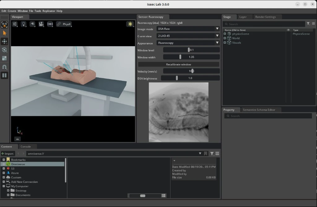 |
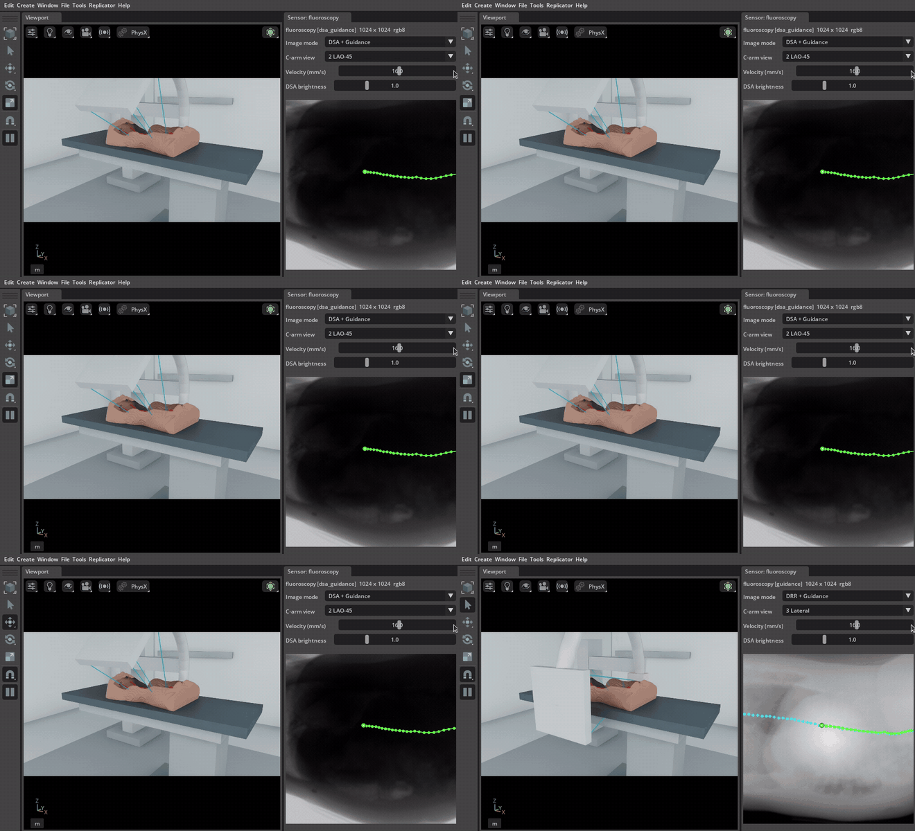
The viewport carries the C-arm, table and patient; the fluoroscopy panel carries the detector image and the controls that drive it. An animated capture shows a C-arm sweep in motion.
Note: Complete the project setup before you begin.
Run with an AI Agent#
Paste any prompt into Claude Code, Codex, or the repository's Local Agent:
Run endoluminal_navigation in demo mode for 1 episode without patient CT data.

Prepare TotalSegmentator sample s0011 as a patient twin.
Run endoluminal_navigation in demo mode and verify fluoroscopy.

Start endoluminal_navigation teleop with the prepared s0011 patient twin.
Run from the Command Line#
Procedural demonstration#
Run the procedural demonstration without patient data:
./run.sh endoluminal_navigation --mode demo
This uses a procedural patient shape, synthetic fluoroscopy, and the default physics settings. The catheter still runs on the Newton rod solver, but with no vessel to contain it.
Patient CT#
Download the public TotalSegmentator small dataset (3.2 GB) and prepare subject s0011:
mkdir -p ./data/TotalSegmentator

curl -L --fail --show-error \
  "https://zenodo.org/records/10047263/files/Totalsegmentator_dataset_small_v201.zip" \
  -o ./data/Totalsegmentator_dataset_small_v201.zip

unzip -q ./data/Totalsegmentator_dataset_small_v201.zip -d ./data/TotalSegmentator
./tools/patient_twin/run.sh ./data/TotalSegmentator/s0011
Preparation reads the CT and its vessel labels through the vasculature_digital_twin package, which resolves each file's own direction cosines and reorients everything onto the canonical LPS patient axes. A study stored feet first, or a label file saved with a different slice order, therefore lands on the same axes as the rest of the twin instead of mirroring the anatomy; the manifest records the frame as DICOM_LPS and metadata.json keeps the orientation the source was stored in. A genuinely oblique acquisition is rejected rather than reoriented, because the renderer samples an axis-aligned voxel grid.
For a subject that ships a CT and no segmentations/ directory, pass --segment-vessels to derive the vasculature with the package's own segmenter instead of reading label files.
Run the demo using the generated manifest:
./run.sh endoluminal_navigation \
  --mode demo \
  --patient-twin ./data/TotalSegmentator/s0011/patient_twin.yaml
Patient-CT fluoroscopy renders with Slang on Vulkan by default. Passing --fluoro-device cuda also needs a CUDA Toolkit on the host (see the requirements); without one, the launcher stops before Isaac Sim starts and names the libnvrtc.so it found, if any.
Keyboard teleoperation#
Launch teleoperation:
./run.sh endoluminal_navigation \
  --teleop \
  --patient-twin ./data/TotalSegmentator/s0011/patient_twin.yaml
Click inside the Isaac window before using the keyboard. The fluoroscopy window provides image, C-arm view, velocity, and brightness controls.
| Keys | Action |
|---|---|
| W / S | Insert / retract catheter |
| A / D | Rotate catheter |
| Z / C | Steer the tip: curl the distal bend either way |
| Q / E | Fine C-arm rotation |
| 1 – 4 | C-arm view presets: AP, LAO-45, Lateral, RAO-30 |
| X | Toggle the simulated contrast (DSA) view |
| R | Reset the catheter and C-arm to their initial state |
| L | Clear a stuck keyboard command |
Fluoroscopy validation#
This mode succeeds only if moving the C-arm changes the fluoroscopy image:
./run.sh endoluminal_navigation \
  --mode validate_fluoroscopy \
  --episodes 2 \
  --patient-twin ./data/TotalSegmentator/s0011/patient_twin.yaml
Recording#
Add --record to store synchronized actions, state, and fluoroscopy frames:
./run.sh endoluminal_navigation \
  --teleop \
  --patient-twin ./data/TotalSegmentator/s0011/patient_twin.yaml \
  --record --record-failures
Recordings are stored under ./runs/endoluminal_navigation/<timestamp>/.
Teleoperation ends the episode when the catheter tip reaches the distal end of the vessel centerline and holds there, so a demonstration is goal-terminated and stored with a success label. Without a patient twin there is no centerline, the criterion can never fire, and the episode runs to the step cap instead. --record-failures additionally keeps attempts that time out for diagnosis. To teach recovery with IL, collect demonstrations that show a successful correction from a wrong branch.
Policy rollout#
Roll out a finetuned GR00T N1.7 checkpoint against the same goal the demonstrations were terminated on:
./run.sh endoluminal_navigation \
  --mode policy_n17 \
  --checkpoint /path/to/checkpoint \
  --patient-twin ./data/TotalSegmentator/s0011/patient_twin.yaml \
  --episodes 10
The mode serves gr00t_n17/catheter_navigation, which declares no published checkpoint, so --checkpoint is required.
Swap the workflow name to roll the same checkpoint out in the arm-borne scene, which serves gr00t_n17/catheter_navigation_arm instead. Both scenes use the same policy groups: catheter, carm, target, and route. The arm's seven servo'd joints are additional recorded state that GR00T does not consume. The arm task is inference-only; recordings from either scene train the shared gr00t_n17/catheter_navigation task.
IL to RL Pipeline and Training Strategy#
Imitation learning (IL) teaches GR00T N1.7 to copy demonstrated velocity commands. Reinforcement learning (RL) then lets that checkpoint interact with the simulator and updates it with PPO according to the navigation reward. These are separate training stages: the remote Task owns IL, and rl/ owns vectorized simulation and online RL outside Workflow run modes.
Teleoperation -> HDF5 recordings -> LeRobot dataset -> GR00T N1.7 IL checkpoint
    -> baseline Isaac Sim evaluation -> RLinf PPO -> native RL checkpoint
    -> RL evaluation -> GR00T export -> policy_n17 evaluation in Isaac Sim
Model inputs and actions#
The current modality configuration consumes a fluoroscopy image, a language instruction, and nine numeric state values:
| Input group | Values | Meaning |
|---|---|---|
video.fluoroscopy |
One image, resized to 256 × 256 by the Task | Current X-ray projection |
state.catheter |
3 | Insertion depth, axial rotation, and tip bend |
state.carm |
1 | C-arm orbit angle |
state.target |
3 | Target minus tip position in world XYZ, in metres |
state.route |
2 | Remaining curved-route distance and tip lateral offset, in metres |
| Language | Task description | What navigation task to perform |
The RL Scene additionally publishes the tip's 3-D position and direction, producing a 15-value environment state. The RL adapter maps only the nine values above into GR00T. The arm's joint positions are not policy inputs.
The four outputs are insertion velocity (m/s), axial rotation rate (rad/s), tip bend rate (rad/s), and C-arm orbit rate (rad/s). They are commands to move the instrument and imaging gantry, rather than desired XYZ tip coordinates. IL predicts 16-step action sequences; the RL configuration uses one action chunk for its PPO policy.
Older checkpoints trained with only catheter and carm state do not have the current target/route contract. Reconvert compatible demonstrations and fine-tune with the current modality configuration and normalization statistics before using those checkpoints with this profile. Changing the input configuration alone does not teach an existing checkpoint to use the new values.
1. Collect and convert demonstrations#
Use a patient twin so recording, goal labels, and reward all refer to the same route. For the intended Franka deployment, collect and validate in endoluminal_navigation_arm, which uses the coupled MJWarp + XPBD solver. Its four command channels match the armless scene, but the carrier arm changes the simulated dynamics.
./run.sh endoluminal_navigation_arm --teleop \
  --patient-twin /absolute/path/to/patient_twin.yaml \
  --record --record-failures
Keep successful, well-controlled demonstrations for the initial IL dataset. Retain failed recordings for diagnosis; blindly copying failed actions does not teach recovery. Demonstrate recovery explicitly when it should become policy behavior.
Inspect the actual HDF5 file, then convert it into a new dataset directory:
RUN_DIR="$(pwd)/runs/endoluminal_navigation_arm/$(date +%Y%m%d_%H%M%S)"
DATASET_DIR="$RUN_DIR/lerobot/local/catheter_navigation"
uv run --project tools/dataset i4h-dataset inspect /absolute/path/to/recording.hdf5 --segments
uv run --project tools/dataset i4h-dataset convert \
  /absolute/path/to/recording.hdf5 "$DATASET_DIR" \
  --robot franka_catheter --repo-id local/catheter_navigation \
  --patient-twin /absolute/path/to/patient_twin.yaml \
  --successful-only \
  --task "Steer the catheter along the vessel and stop at the target branch"
For armless recordings, use --robot catheter. The converter derives the five target/route columns from the recorded tip trajectory and the twin's route. It requires the diagnostics/tip_world_m trajectory; an old recording without that trajectory cannot supply these columns merely by naming a patient twin. Verify nonzero episode count, camera videos, episode parquet files, and meta/info.json, meta/stats.json, and meta/modality.json before training.
The converter also accepts multiple HDF5 inputs before the output path. This allows recordings of subjects s0058, s0223, and s0250 to share one dataset and normalization statistics. For that case, omit --patient-twin: each recording must have a sibling run.json identifying its own twin. Do not assign one anatomy's route to all three subjects. Use recordings from the same embodiment descriptor in one conversion.
2. Fine-tune and evaluate GR00T N1.7#
Both embodiments train the shared catheter Task. Resolve the configuration first:
uv run --project tasks/gr00t_n17 i4h-tasks-gr00t-n17-train \
  --task gr00t_n17/catheter_navigation \
  --dataset "$DATASET_DIR" --output-dir "$RUN_DIR/il_checkpoints" \
  --max-steps 10000 --save-steps 1000 --batch-size 32 --num-gpus 1 \
  --dry-run
Remove --dry-run to train. These example values match the Task defaults: base model nvidia/GR00T-N1.7-3B, 10,000 optimizer steps, and checkpoints every 1,000 steps. The training wrapper defaults to learning rate 1e-4, training the projector and diffusion model while leaving the language backbone and vision tower frozen. The resolved dry-run output is the authority for an individual run.
Select an actual saved checkpoint directory and establish a baseline with the policy rollout command, using the arm workflow for arm deployment. Compare success, final route distance, and wall behavior across repeated episodes. A lower IL loss means closer agreement with demonstration commands; it does not establish navigation success.
3. Post-train with RLinf PPO#
The arm profile selects RLinf and requires a patient twin plus a compatible local IL checkpoint. Preview it, then resolve a short, one-anatomy smoke run:
./train.sh rl show endoluminal_navigation_arm
./train.sh rl endoluminal_navigation_arm \
  --model-path /absolute/path/to/il_checkpoint \
  --patient-twin /absolute/path/to/patient_twin.yaml \
  --num-envs 1 --epochs 2 --dry-run
Remove --dry-run to run. For a training run, choose the environment count and epoch budget explicitly. Logs and checkpoints go under runs/endoluminal_navigation_arm/<timestamp>/; --run-dir can name a new directory in that layout.
Profiles default to model GPU 0 and simulator GPU 1, with separate Python processes to isolate their dependencies. A single GPU is supported by prefixing the command with I4H_RL_SIM_GPU=0; model, simulation, and rendering then share its memory. The defaults of four arm environments and eight armless environments are starting estimates, not measured hardware limits. Measure memory and step throughput before raising them.
The current PPO configuration uses:
| Parameter | Default | Interpretation |
|---|---|---|
| PPO epochs | 500 | Maximum outer collection/update cycles |
| Rollout batches per update | 8 | Collect all eight before a PPO update |
| Steps per rollout / episode budget | 600 | At most 20 seconds of simulated control time at 30 Hz |
| PPO passes | 4 | Reuse the collected batch for four optimizer passes |
Discount gamma / GAE lambda |
0.995 / 0.95 | Weight future reward and smooth advantage estimates |
| Policy / value learning rate | 5e-6 / 1e-4 |
Update the action policy slowly and its reward predictor faster |
| PPO clip ratio | 0.2 | Limit the change in action probability |
| Micro / global batch size | 2 / 240 | Per-device working batch and optimizer batch size |
| Precision / training backend | bf16 / FSDP | Model arithmetic and parameter handling |
| Checkpoint interval | 2 | Save every two outer epochs |
With N environments, a collection cycle has a configured budget of 8 × 600 × N environment steps. Global batch size must divide the trainer's collected sample count; action chunking affects how those samples are represented. Slow wall-clock rollout time is possible even though an episode represents only 20 simulated seconds.
Dense reward: advance, follow the route, avoid the wall#
The reward quantities are implemented in navigation_reward.py. Their weights and the final three-term wiring are in navigation_rewards_cfg. Isaac Lab's reward manager sums the weighted terms with control-step time scaling:
delta_s = clamp(previous_remaining - current_remaining, -0.0025, +0.0025)
lateral_cost = max(tip_lateral - 0.5 * local_lumen_radius, 0) / local_lumen_radius
wall_depth = max_over_rod_particles(max(particle_lateral - local_lumen_radius, 0))

reward = dt_control * (400 * delta_s - 0.1 * lateral_cost - 400 * wall_depth)
dt_control = 1/30 second
| Term | Simple meaning | How to interpret it |
|---|---|---|
route_progress |
Pay for moving forward along the curved vessel | Forward progress is positive, retreat is negative, standing still earns zero. The ±2.5 mm clamp limits reward from jumps in nearest-route projection. |
lateral |
Charge for straying too far from the planned centerline | The inner half of the local radius is free. Beyond it, the cost grows with deviation relative to vessel size. |
penetration |
Charge for the deepest rod point outside the modeled lumen | Measures the whole catheter, including the shaft. A 2.5 mm violation cancels a maximum-scale progress term for that step before the lateral cost. |
Remaining distance is measured along an ordered 3-D centerline polyline, including its curves. The shared route builder resamples the route at 7.5 mm spacing for both simulation and dataset conversion. The tip is projected onto the nearest segment, and remaining arc equals total route length minus the projected arc position. These sampled points describe one continuous route; the policy is not rewarded for reaching discrete waypoints in sequence. At bifurcations, the selected route encodes the intended branch. Reward can favor that route, but the policy must also receive useful goal cues and demonstrations to steer into it.
The wall cost approximates the lumen with route points and local radii; it is not a tissue-damage model. If radii are absent, both lateral and penetration weights are zero. No approach bonus, arrival bonus, fold flag penalty, or action-rate penalty is configured. Reward is feedback used during training, rather than another observation passed to GR00T.
Success is a separate termination criterion: the tip must stay within the configured straight-line target tolerance for 15 consecutive control steps (about 0.5 seconds). The endoluminal default is 8 mm, overridable with I4H_CATHETER_ARRIVAL_MM; the generic medical helper defaults to 5 mm. Keep the same tolerance when collecting, training, and comparing evaluations. The 600-step budget is a timeout/truncation, not success. High route progress alone cannot establish arrival or safe navigation.
Monitoring in TensorBoard and Weights & Biases#
Open the run's events using the TensorBoard installation in the GR00T environment:
tasks/gr00t_n17/.venv/bin/tensorboard \
  --logdir /absolute/path/to/rl_run/tensorboard --port 6006
Look in Scalars (or the scalar cards in the Time Series view). The rollout monitor flushes metrics after each completed rollout batch, while PPO loss appears only after all eight batches and the optimizer update. Its scalar step is the total completed rollout count. Values describe completed batches, not live tip motion between them.
| Metric | Meaning | Useful interpretation |
|---|---|---|
monitor/success_rate |
Fraction of environments that satisfied arrival at least once in that batch | Zero means no observed arrival; it does not mean zero movement. With one environment the batch value is 0 or 1, so compare many batches. |
monitor/mean_return |
Mean accumulated reward across environments | Compare trends with the same anatomy, weights, tolerance, and horizon. Higher can mean better progress or fewer costs; it is not itself success. |
monitor/mean_reward |
Mean of accumulated reward divided by elapsed steps | Average reward per step, rather than total episode return or an individual reward term. |
monitor/mean_episode_length |
Mean elapsed episode steps in the adapter | Reaching the budget with zero success suggests timeout. Interpret alongside success because a shorter run alone need not be better. |
monitor/rollout_index, monitor/progress_fraction |
Position within the eight batches for the current update | Confirms collection is advancing; resets its cycle after each update. |
monitor/rollout_duration_seconds, monitor/estimated_seconds_to_update |
Measured batch duration and estimated remaining collection time | Throughput indicators; the estimate does not include the upcoming PPO optimization time. |
| PPO policy/value losses and optimizer statistics | Policy update size and error in predicted return | Useful for diagnosing unstable updates. Their decline alone does not prove the catheter is reaching the target. |
rollout_progress.json in the run directory provides the same small batch-progress summary for external monitoring. A process being alive, a monitor event file, and a successful rollout are different observations. For assessing learning, prioritize success over repeated evaluations, remaining curved-route distance, lateral deviation, and wall penetration. The latter geometry diagnostics must be read from available simulator logs or explicitly added as metrics; the monitor above does not currently emit them.
During PPO optimization, rollout_progress.json stays at rollouts_complete_waiting_for_optimizer until collection resumes. Follow the actor log for PPO optimization started and one PPO optimizer step ... finished line per step, including the count within the current update and elapsed seconds. GR00T N1.7 actor and rollout workers install the same linear Qwen3-VL patch embedding used by fine-tuning and inference, avoiding the slow bf16 Conv3d path while preserving checkpoint parameters and gradients. Existing checkouts should rerun ./third_party/setup.sh tasks/gr00t_n17 to apply the worker patch before restarting training.
RLinf defaults to TensorBoard. After authenticating with tasks/gr00t_n17/.venv/bin/wandb login, enable both trainer backends with the additional argument --set 'runner.logger.logger_backends=[tensorboard,wandb]'. The custom monitor/* writer remains a TensorBoard writer; enabling the trainer's W&B backend does not automatically mirror that writer's scalars.
Anatomy curriculum, evaluation, and checkpoint handoff#
Start with an IL baseline and a short one-anatomy RL run to verify compatible inputs, finite rewards, PPO updates, and saved checkpoints. Then evaluate whether progress improves without increasing wall violations. For Franka deployment, include the arm scene in both training and evaluation even when an armless run is useful for faster diagnostics.
The current RL launcher takes one --patient-twin per run; increasing --num-envs creates more environments on that same anatomy. To continue across s0058, s0223, and s0250, run explicit stages and use --resume-dir /absolute/path/to/previous_rl_run with the same compatible --model-path. Resume restores training state; it is not automatic per-episode anatomy sampling. Sequential anatomy stages can forget earlier subjects, so re-evaluate all training subjects after each stage and reserve additional anatomies for held-out evaluation. Mixed-anatomy IL data can provide a broader initialization before this sequence.
RLinf saves native actor weights under actor/model_state_dict/full_weights.pt inside its checkpoints. On successful completion, the wrapper writes checkpoint.json in the run directory to identify the latest weights, base checkpoint, and trainer configuration. Those native weights need export before normal GR00T Workflow serving:
./train.sh rl endoluminal_navigation_arm --eval \
  --checkpoint /absolute/path/to/rl_run \
  --patient-twin /absolute/path/to/patient_twin.yaml --num-envs 1

./train.sh rl export endoluminal_navigation_arm \
  --checkpoint /absolute/path/to/rl_run \
  --output-dir /absolute/path/to/exported_gr00t_checkpoint

./run.sh endoluminal_navigation_arm --mode policy_n17 \
  --checkpoint /absolute/path/to/exported_gr00t_checkpoint \
  --patient-twin /absolute/path/to/patient_twin.yaml --episodes 10
Use the run directory containing checkpoint.json, or a supported native checkpoint path with its corresponding configuration. Inspect the evaluation output and visibly validate the exported policy in Isaac Sim; written checkpoint files alone do not demonstrate task success. Keep the physics setup, solver revision, arrival tolerance, input contract, and patient twin traceable with the run artifacts.
Validate checkpoints and check whether the policy is learning#
Checkpoint validation has two parts: confirm that inference can load the model, then measure what it does in the simulator. Apply both to the IL checkpoint and to each selected RL checkpoint after export.
First, run a load check through the actual GR00T serving backend. Set CHECKPOINT to the IL checkpoint directory or the exported RL checkpoint directory:
CHECKPOINT=/absolute/path/to/gr00t_checkpoint
uv run --project tasks/gr00t_n17 python -m i4h_tasks.gr00t_n17.server \
  --namespace catheter-checkpoint-smoke \
  --preload gr00t_n17/catheter_navigation_arm \
  --checkpoint "$CHECKPOINT" --preload-only
A successful exit confirms model loading; the simulator rollout still needs to verify that the observation/action contract works and the catheter navigates. Run repeated episodes and retain failures so that the recordings show the complete evaluation rather than only successful attempts:
EVAL_RUN="$(pwd)/runs/endoluminal_navigation_arm/$(date +%Y%m%d_%H%M%S)"
./run.sh endoluminal_navigation_arm --mode policy_n17 \
  --checkpoint "$CHECKPOINT" \
  --patient-twin /absolute/path/to/patient_twin.yaml \
  --episodes 20 --record --record-failures --run-dir "$EVAL_RUN"
Repeat this for an early and a later IL checkpoint, then for the initial IL checkpoint and selected exported RL checkpoints. Use fresh evaluation directories. Compare the same anatomies, initial conditions, sampling settings, solver revision, control rate, arrival tolerance, and 600-step budget. Repeat on held-out anatomies as well as training subjects. Twenty episodes is a useful first comparison, not a guarantee of a reliable success estimate; repeated identical deterministic episodes only test repeatability, so include varied valid starts or additional subjects when assessing robustness.
For a native RL checkpoint, also run the RLinf --eval command in the previous subsection. It performs evaluation without PPO updates and writes evaluation.json containing eval/success_once, eval/return, eval/episode_len, and eval/num_trajectories. For RLinf, --episodes is not an episode-count control; evaluation volume comes from the environment count and evaluation rollout configuration. Read the reported trajectory count. The wrapper reports failure when no task success is observed, even if the simulator completed its evaluation normally.
| Comparison | Evidence of improvement | What it does not establish |
|---|---|---|
| Arrival success across matched evaluation episodes | A higher fraction reaches and holds at the target | One lucky success does not establish reliable navigation |
| Final remaining route distance, including failed episodes | Less vessel remains when success is still zero | Minimum distance reached once can hide retreat or unstable motion |
| Lateral offset and deepest wall penetration over the trajectory | More progress with equal or lower deviation and penetration | Shorter route distance achieved by cutting through the wall is not an improvement |
| Completion steps among successful episodes | Reaches and holds sooner with similar wall behavior | A short failed or prematurely stopped episode is not better |
| Performance on held-out anatomies | Gains extend beyond the training route | Better performance on one training subject may be memorization |
Use simulator readouts and recorded trajectories to assess the geometry rows; they are not all automatically included in monitor/* or evaluation.json. Report both the number of successful episodes and the number evaluated, and preserve timeout/failure results. A reward increase is useful supporting evidence only when the reward configuration is unchanged and wall behavior also improves.
For IL, falling training loss means the model better matches training demonstrations. Check simulator behavior and performance on demonstrations or anatomies excluded from training to see whether that improvement generalizes. For RL, falling PPO or value loss means the optimizer is fitting its collected data; compare independent evaluation runs against the unchanged IL baseline to establish navigation improvement. If success remains zero but remaining route distance decreases without higher lateral offset or penetration, that is measurable partial progress. If those quantities and success are unchanged across several checkpoint evaluations, the losses alone do not support a claim that navigation is improving.
For a real procedure, target offset and route distances require a registered anatomical plan and a compatible estimate of the tip's 3-D position. A fluoroscopy image alone does not directly supply these simulator values. Match the observations available on the real system before deploying a policy trained with them.
Unified Simulation Loop#
The loop is unified in the sense that three separately maintained packages act on one anatomical domain, through one coordinate chain, advanced by one owner of time. No stage re-derives the anatomy for its own use.
| Stage | Artifact it owns | Role in the loop |
|---|---|---|
vasculature_digital_twin, through PatientTwin |
mu_volume.npy, metadata.json, centerline graph, vessel mask, anatomy USD |
Attenuation field, insertion path, and the transforms every other stage is expressed in |
catheter_vasculature_solver.CathRodSolver |
node positions and orientations in solver-local metres | Advances the rod under Cosserat stretch and Darboux constraints, plus its projections |
xray_simulator Slang DiffDRR, with CatheterAttenuation |
the detector image | Marches CT attenuation and catheter attenuation into one Beer-Lambert exponent |
arena/i4h_arena/runner.py is the only caller of env.step, and immediately after each step it invalidates the single read cache that the fluoroscopy window, the recorder, and the publisher all read through. That is what makes a recorded step self-consistent: the image, the action, and the joint state describe the same simulator state rather than three states a frame apart.
Notation used below:
x_i, q_i    node position (solver-local metres) and orientation (unit quaternion), i = 0..N
l, N, r     segment rest length, segment count, rod radius
mu          attenuation field [1/mm] on the twin's ZYX voxel grid, trilinearly sampled
gamma(s)    centerline by arclength, [0, L_path] -> world metres
s           insertion arclength of the rod's proximal end
A           affine transform, volume millimetres -> world metres
theta       C-arm orbit angle
h           XPBD substep; dt_phys physics step; dt_ctrl control step
Rates, and what runs in lockstep#
| Period | Value | Set by |
|---|---|---|
Control step dt_ctrl |
1/30 s | env_cfg.decimation = 4 over sim.dt |
Physics step dt_phys |
1/120 s | env_cfg.sim.dt |
XPBD substep h |
1/120 s | One rod substep per physics step: NewtonCfg.num_substeps and XPBDRodSolverCfg.num_substeps both default to 1 |
| Fluoroscopy frame | 1/15 s | FluoroscopySensorCfg.update_period |
| Viewport render | 1/30 s | env_cfg.sim.render_interval = 4 |
The nesting is exact rather than approximate: one action is clamped once per control step and then applied on all four physics steps of that step, and each physics step advances the rod by one XPBD substep inside Newton. Four substeps therefore separate two consecutive actions. Imaging is not part of that chain — the sensor is pulled, not pushed, so when the 1/15 s period has elapsed it takes a fresh CatheterState snapshot and a fresh CArmState at that instant. A frame is never composed from a stale polyline and a current C-arm pose, and no frame is rendered twice.
One control step is the composition
I_k = Psi . R_theta_k . T . (Phi^dt_phys)^4 (X_{k-1}, s_{k-1}, u_k)
with Phi the physics advance, T the geometry handoff, R_theta the fused projection, and Psi the display mapping. Psi is the only stage whose settings a live operator can change, which is why it is also the only stage excluded from the recorded attenuation channel.
UNIFIED_SIM_LOOP(mu, gamma, A)                     # runner.py owns env.step
  precompute   mu, gamma, A                        # patient twin, offline
  initialise   X_0 = (x_0, q_0, v = 0, w = 0)
               s_0 = 0,  theta_0 = 45 deg
  for k = 1, 2, ...
      u_k = (v_ins, tau, bend_rate, orbit_rate)    # keyboard/UI -> action tensor
      for j = 1..4                                 # decimation, one XPBD substep each
          (X, s) <- Phi^dt_phys(X, s, u_k)
          theta  <- clip(theta + orbit_rate*dt_phys, -30 deg, +90 deg)
      S_k <- T(x)                                  # spans in volume millimetres
      if the sensor period has elapsed
          I_k <- Psi( R_theta( mu (+) S_k ) )
      display and record (u_k, joint state, I_k) through one invalidated view
Precompute: the patient twin#
./tools/patient_twin/run.sh maps Hounsfield units to a linear attenuation coefficient with a piecewise-linear curve, clamped outside its outer knots:
mu(HU) = mu_j + (HU - HU_j) * (mu_{j+1} - mu_j) / (HU_{j+1} - HU_j)     HU in [HU_j, HU_{j+1}]
mu(HU) = mu_0                                                          HU <= HU_0
mu(HU) = mu_M                                                          HU >= HU_M
The default interventional preset uses knots (-1000, 0), (-300, 0), (100, 0.0008), (300, 0.0028), (500, 0.0060), (900, 0.0090), (1500, 0.0120), (3000, 0.0200), (8000, 0.0440) in HU and 1/mm. Soft tissue is deliberately suppressed relative to the two-knot linear ramp, because a fluoroscopic beam barely sees it, while contrast, cortical bone, and implant density each keep a slope of their own. The knots are written into metadata.json under hu_to_mu, so a twin is traceable to the curve that built it and an episode cannot silently mix two attenuation models.
Three frames meet in the manifest, and the composition is what keeps the renderer, the solver, and the USD stage from disagreeing:
voxel -> patient mm     V = voxel_to_patient_mm         # spacing, origin, direction cosines
patient mm -> world m   W . S,  S = diag(1e-3,1e-3,1e-3,1)
voxel -> world m        A_voxel = W . S . V
volume mm -> world m    A = A_voxel . diag(1/spacing_xyz, 1)
world m -> volume mm    A^-1                            # the handoff T
The centerline arrives as a graph rather than a path. ordered_centerline_path recovers the primary vessel by running Dijkstra between degree-one endpoints with edge weights |p_a - p_b| / sqrt(mean radius), which biases the path into large vessels rather than into whatever branch happens to be longest, starts from the most caudal endpoint, smooths the result with a [1/4, 1/2, 1/4] stencil, and resamples it uniformly at 7.5 mm. Arclength is the cumulative chord length of that polyline. The rod's initial length is L_path - 0.12 m (route_initial_catheter_length_m), so every twin leaves the same 120 mm of route to insert within the 600-step budget; a route shorter than that allowance is seeded nearly whole.
For the s0011 twin this yields a 431x311x311 grid at 1.5 mm isotropic spacing (646.5 x 466.5 x 466.5 mm), mu in [0, 0.0234] 1/mm, a 646 mm route and so a rod of about 526 mm, divided into N = 120 segments (DEFAULT_NUM_SEGMENTS) so l is about 4.4 mm, and r = 0.5 mm.
Control#
Keyboard and UI input becomes one action tensor per control step: three components for the catheter and one for the C-arm. CatheterVelocityAction clamps insertion to +/-0.060 m/s, axial rotation to +/-1.5 rad/s, and the tip bend rate to +/-1.5 rad/s, integrating the last into a tip bend angle held within +/-1.5 rad. The panel's velocity slider spans 1 to 60 mm/s and defaults to 9 mm/s, because a sustained 30 mm/s feed drives the shaft through the wall on this scene. CArmOrbitAction clamps the orbit rate to +/-0.6 rad/s and integrates it into an angle bounded to [-30, +90] degrees, starting at 45. The runner additionally refuses to step on a non-finite action, which localises a bad command to the step that produced it.
Physics advance#
With a patient twin only the proximal end is prescribed; the rest of the rod is solved:
Phi^dt_phys(X, s, u)                                # CatheterVelocityAction.apply_actions
  s <- clip(s + v_ins*dt_phys, ...)                 # RouteRailedIntroducer: arc length is the state
  x_0, q_0 <- gamma(s), twist(tau)                  # place_proximal; the root has zero inverse mass
  beta <- clip(beta + bend_rate*dt_phys, -1.5, 1.5) # set_tip_bend
  X <- S^h(X)                                       # one XPBD substep inside Newton
The rod's shape is seeded from the centerline once, at reset, and is not resampled afterwards. The drive integrates insertion into the root's arc length along the route and places the root there, so it stays on the vessel however long insertion is held and a command the route cannot take is not recorded as insertion.
Track guidance holds the shaft that has already been traversed onto the route, and leaves a free distal window of 1.5 times the 120 mm insertion allowance. Inside that window the shaft and tip are governed by the constraint solve and by containment against the twin's deformable vessel wall. Axial rotation turns the material frames, and with them the plane the tip bend curls in. Without a twin there is no route or vessel: the root is fed along its own tangent and the rod moves freely.
One XPBD substep#
S^h(X)                                              # XPBDRodSolver._substep
1 predict      v <- (1 - d)(v + h(M^-1 f + g)),  x* <- x + h v
               w <- (1 - d)(w + h I^-1 tau),     q* <- normalize(q + (h/2)(w,0) . q)
               x*_i <- x_i, v_i <- 0  where  1/m_i = 0          # kinematic nodes
2 pre-project  x* <- Pi_M(x*)                       if enabled  # off in this workflow
3 compliance   a_str = 1e-10                                    # near-inextensible
               a_bend = 1/(E b_x l h^2 + eps), 1/(E b_y l h^2 + eps)
               a_twist = 1/(G b_z l h^2 + eps)
4 solve        x*, q* <- C(x*, q* ; a)
5 post-project x* <- Pi_A(x*)  then  Pi_M(x*)       if enabled
6 integrate    v <- (x* - x)/h,  x <- x*
               w <- 2 Im(q* . q^-1)/h,  q <- q*
g is zeroed for this scene, since a catheter inside a vessel is not a falling rod. The material defaults are E = 1e9 Pa, nu = 0.3 so G = E/(2(1+nu)) = 3.85e8 Pa, bend multiplier b_x = b_y = 0.1, twist multiplier b_z = 0.4, and d = 0.01 per substep. Compliance is inversely proportional to h^2, so it is the substep and not the control rate that sets the effective stiffness. The damping is per substep, so 0.01 at 120 Hz removes roughly 70% of residual velocity per second, which is the role the standalone viewport gives its per-frame 0.82 dissipation factor.
The steerable tip is a rest shape rather than a force. Every physics step, set_tip_bend(beta) writes a rest Darboux vector (sin(beta/(2 n_tip - 1)), 0, 0) onto each of the last n_tip edges, so the bend constraint drives the tip polyline toward a turn of beta about the tip's local X axis and the solver resists straightening it. beta is the tip bend angle integrated from the Z/C rate command, and n_tip covers tip_length_m = 25 mm rounded up to whole segments, six at the s0011 segment length. Axial rotation aims the bend at a branch.
The Cosserat constraint solve#
C(x*, q* ; a)                                       # per edge i, 6 rows
  r_0 = R(q*_i)(0, 0, +l_i/2)
  r_1 = R(q*_{i+1})(0, 0, -l_i/2)
  C_str = (x*_i + r_0) - (x*_{i+1} + r_1)                       # stretch and shear
  C_dar = Im(q*_i^-1 . q*_{i+1}) - u_rest_i                     # bend and twist
  dC_str/dx = [ +I3, -I3 ],   dC_str/dtheta = [ [r_0]x, -[r_1]x ]
  W = diag( w_i I3,  R I~^-1 R^T )
  ( J W J^T + diag(a) ) dlambda = -C - diag(a) lambda           # 6x6 block tridiagonal
  lambda <- lambda + dlambda
  x*_i  <- x*_i + W_x J_x^T dlambda
  q*_i  <- normalize( q*_i + (1/2)(W_theta J_theta^T dlambda, 0) . q*_i )
The system is block-tridiagonal because each edge couples only its two adjacent nodes, so it is solved directly by a block Thomas recursion over 6x6 blocks rather than by Gauss-Seidel sweeps. A direct solve is what lets a near-inextensible rod hold its length in a handful of substeps; an iterative solve at the same budget visibly stretches under a push.
Projections#
Both projections are implemented in the solver package and both are position-level, applied to predicted positions before the substep integrates:
Pi_M(x*)  vessel containment                        # BVH signed-distance query
  phi = sigma |x*_i - c|,  n = sigma (x*_i - c)/|x*_i - c|      # c = closest surface point
  if phi > phi*                                                # phi* = -r, a clearance shell
      p = x*_i - n (phi - phi*)
      if <p - x_i, n> > 0:  p <- p - n <p - x_i, n>             # forbid outward motion
      x*_i <- p
  repeated collision_iterations times; wall friction may then damp tangential velocity
  on the contact band, which is off by default

Pi_A(x*)  track guidance                            # non-tip nodes only
  t = clamp( <x*_i - a, d>, 0, L_track )
  x*_i <- x*_i + kappa ( a + t d - x*_i ),  kappa = 0.65
In this workflow the static-mesh form of Pi_M stays off (collision_enabled=False). With a patient twin, containment instead runs against a deformable vessel built from the twin's centerline and lumen radii, inside the rod solver's own kernels, alternating with the elastic solve for contact_coupling_iterations = 32 rounds per substep. Running both would apply two independent wall constraints to the same catheter. Pi_A runs as track guidance on the shaft already traversed, leaving the free distal window described under Physics advance. Without a twin, neither runs.
Geometry handoff#
T(x)                                                # CatheterAttenuation input
  p_i = A^-1 x_i                                    # world metres -> volume millimetres
  spans = { (p_i, p_{i+1}) : i = 0..N-1 },  |p_{i+1} - p_i| > 1e-6
  radius = 1000 * CatheterState.radius_m
  d_i = sum_{j >= i} L_j - L_i/2                    # arclength from the tip to span midpoint
  mu_i = mu_tip   if d_i <= tip_length_mm  else  mu_shaft
The transform is the inverse of the twin's declared affine, so a study with non-trivial direction cosines lands correctly instead of relying on a hardcoded rebase. The radius comes from the physics side, so the image and the mechanics cannot disagree about how thick the instrument is, and the tip band is assigned by arclength rather than by a fixed number of spans, whose length depends on the solver's segment count.
Image formation#
solve_projection_geometry converts Isaac world poses into the renderer's centred volume frame: it builds an orthonormal detector basis from the source-to-detector axis, takes SID = SDD/2, places the isocenter at source + SID * beam, expresses the translation as isocenter - volume centre, and inverts the renderer's Rz Rx Ry Euler convention. Square detector pixels are required and non-square input is rejected rather than silently stretched. The scene gives SDD = 1020 mm, SID = 510 mm, so magnification M = SDD/SID = 2, and a 0.6144 m detector over 1024 pixels gives a 0.6 mm pitch, a 614.4 mm field of view, and 0.3 mm ray spacing at the isocenter.
R_theta(mu (+) S)                                   # per detector pixel (u,v)
  src = T_theta(0, 0, -SID)
  det = T_theta( (u + 1/2 - n_u/2) pitch,  (v + 1/2 - n_v/2) pitch,  SDD - SID )
  e   = normalize(det - src),   span = |det - src|
  [t0, t1] = RayBox(src, e, Omega)                  # slab method on the volume AABB
  if the ray misses:  I(u,v) = I0;  continue
  Sigma_vol = sum_j mu( src + e (t0 + (j + 1/2) ds) ) ds        # midpoint, trilinear
              j = 0 .. floor((t1 - t0)/ds),  capped at 2048 steps
  Sigma_cat = sum_i mu_i * chord(src, e, p_i, p_{i+1}, r, span)
  I(u,v) = I0 exp( -(Sigma_vol + Sigma_cat) )
Beer-Lambert is additive in the exponent, which is the whole reason the catheter can be a separate solve without ceasing to be part of the beam: the code multiplies exp(-Sigma_vol) by exp(-Sigma_cat), and that product is the single fused line integral. Occlusion by dense bone, cone-beam magnification, and foreshortening where the shaft runs along the beam then all follow from the geometry instead of being painted on.
The catheter chord is solved analytically per span rather than sampled. With e_axis the span direction, d_perp and f_perp the components of the ray direction and of src - p_i perpendicular to it:
|d_perp|^2 t^2 + 2 <d_perp, f_perp> t + (|f_perp|^2 - r^2) = 0   -> [t_enter, t_exit]
t clipped to the two end planes  (0 - f_axis)/d_axis, (L - f_axis)/d_axis
t clipped to [0, span]                                          # between source and detector
chord = max(0, t_exit - t_enter)
Two details differ from a literal reading of the reference shader. Chords are analytic because a 0.5 mm shaft is thinner than the 1.0 mm march step and sampling aliases it in and out of view along its length. And spans end flat rather than rounded, so consecutive spans meet at a shared plane instead of overlapping and double-counting material where nodes sit a fraction of a millimetre apart; what that leaves unmodelled is a wedge on the outside of each bend of order r * half-angle, well under a pixel at these scales.
Contrast is a second render, not an overlay: mu is copied, multiplied by dsa_boost = 6 inside a centerline mask dilated to 1.2 mm, and marched with the same pose and the same catheter factor. The cyan vessel tint is derived from the difference of the two transmissions, normalised by its 99.5th percentile and capped at 0.82 alpha.
Display mapping#
Psi(I)                                              # xray_simulator.display
  t = I / I0,   p = -ln clip(t, eps, 1)             # back to the line integral, floored
  s = 1 - clip( (p - p_lo)/(p_hi - p_lo), 0, 1 )
  g = s              for polarity "fluoro"
  g = 1 - s          for polarity "diagnostic"
  g = clip(g,0,1)^(1/gamma)
  8-bit image = round(255 g)
  attenuation channel = 1 - t                       # float32, before any of the above
The window is fitted once, from the first frame, as the 1st and 99th percentiles of p with the low end clamped at zero, and then held fixed so that brightness reflects the anatomy in the beam rather than the frame's own range. The two sliders move that fitted window relatively, which is why the same bounds suit any patient:
W_0 = p_hi_0 - p_lo_0
c   = (p_lo_0 + p_hi_0)/2 + level * W_0             # level in [-1, 1]
W   = max(W_0 * width, 1e-6)                        # width in [0.25, 4]
p_lo = max(c - W/2, 0),   p_hi = p_lo + W           # a line integral cannot start below zero
The cinematic style adds a 0.9 px blur, a 0.85/0.15 mix with a 2.2 px bloom, 0.76/0.24 temporal persistence, Gaussian noise at sigma 0.012, and a vignette with a 1.06 gamma. Like everything else in Psi it touches the displayed image only, never the attenuation channel.
Fluoroscopy Image Appearance#
The renderer produces transmission exp(-∫μ ds), so dense anatomy carries less signal than air. Two settings decide how that becomes pixels.
| Setting | Default | Effect |
|---|---|---|
| Appearance dropdown in the fluoroscopy panel | Fluoroscopy |
Fluoroscopy draws bone, contrast and the catheter dark on a bright background, as on a cath-lab monitor. X-ray inverts it for the film-radiograph look. Also settable in code as FluoroscopySensorCfg.display_polarity (fluoro or diagnostic) to fix the look for a headless or recorded run. |
| Window level and Window width sliders | 0.0 and 1.0 |
Contrast control, in multiples of the window fitted from the first frame. Narrowing the width raises contrast and clips dense structures earlier; the level shifts the whole tone curve. |
| Recalibrate window button | — | Re-fits the window to the next frame and returns both sliders to neutral. |
./tools/patient_twin/run.sh --hu-to-mu |
interventional |
Attenuation curve baked into the twin. interventional suppresses soft tissue and keeps implant density separated from cortical bone; linear reproduces twins built before named curves existed. |
Everything in the first three rows is a re-map of the frame already in hand rather than a re-render, so it applies instantly and cannot disturb a run. Polarity only decides which way round the greys go, and switching it preserves the calibrated window, so brightness stays comparable between the two looks. The synthetic CI phantom has no display mapping and keeps its fixed appearance.
Brightness comes from a display window measured once from the first frame of a run and then held fixed, so moving the C-arm or advancing the catheter changes the image only where the anatomy in the beam actually changes. Rescaling every frame by its own range would instead tie background brightness to whatever is in the field of view, which flickers through a sweep and gives a policy a moving target. That fit reflects whatever was in the beam at step zero, which is why a large oblique or a move along the table may warrant Recalibrate window. The sliders are expressed as multiples of the fitted width rather than in absolute line-integral units so that the same bounds suit any patient, since the useful range depends on body size and on the μ scaling baked into the twin.
The attenuation curve is deliberately not adjustable at runtime. It is baked into mu_volume.npy when the twin is built and uploaded as a GPU volume texture, so changing it means re-running the preprocessor over the whole CT and rebuilding that texture. More importantly it is the twin's physical identity, recorded under hu_to_mu in its metadata.json, and a live control would let one episode contain frames from several different attenuation models. Rebuild the twin with --hu-to-mu to change it; use the window sliders for the viewing-time effect.
What Recordings Store#
--record writes two channels per fluoroscopy frame. obs/fluoroscopy is the 8-bit image as displayed, which folds in polarity, window and gamma, and is what a human or a VLM annotator should look at. obs/fluoroscopy_attenuation is the float32 1 - exp(-∫μ ds) the renderer produced, before any display mapping, and is therefore reproducible no matter how the live view was set while recording. Prefer it for training and for anything that has to be comparable across runs. It costs roughly a third more space per frame than the image, so expect recordings to grow accordingly.
Catheter Appearance#
The catheter is part of the beam, not an annotation. Each span between solver nodes is a cylinder with its own attenuation coefficient, and its contribution is added to the line integral of the volume behind it — the same fused Beer-Lambert march the interactive catheter viewport performs in its shader. So the instrument is occluded by dense bone instead of covering it, grows as it approaches the detector, foreshortens into a blob where it runs along the beam, and reaches the attenuation channel that rewards and policies read.
| Setting | Default | Effect |
|---|---|---|
FluoroscopySensorCfg.catheter_attenuation |
True |
Composite the catheter into the beam. Setting it to False restores the previous behaviour, a flat dark polyline drawn onto the finished image. |
FluoroscopySensorCfg.catheter_shaft_mu_per_mm |
0.8 |
Shaft attenuation, in the range of braided nitinol. |
FluoroscopySensorCfg.catheter_tip_mu_per_mm |
3.0 |
Marker band at the distal tip, in the range of tungsten-loaded polymer. This is the cue an operator uses to find the tip. |
FluoroscopySensorCfg.catheter_tip_length_mm |
2.0 |
Length of the distal end carrying the marker coefficient. |
The shaft's diameter comes from the physics side, as CatheterState.radius_m, so the image and the mechanics cannot disagree about how thick the instrument is. The green path in the guidance stream stays an overlay: rgb and dsa are what a detector would measure, guidance and dsa_guidance add annotation on top.
Current Limitations#
This is an integration demonstration, not validated intravascular mechanics. There is no dose model, the C-arm is single-plane rather than biplane, and the only Zenoh traffic is the remote-task link policy_n17 uses to reach its policy server. The green catheter guidance is presentation-only.
The vessel wall is a deformable vessel built from the twin's centerline and lumen radii, not the segmented vessel surface, and it is not a tissue model: it keeps the rod inside the lumen without modelling vessel injury. The solver's static-mesh collision path is unused. Containment is a projection, so the rod can still end up partly outside the lumen; the RL reward measures that against the same radii and penalises it.
The rod physics runs batched across environments. Patient fluoroscopy does not: the pinned xray_simulator release behind the Slang renderer supports one environment, and it raises on a batch rather than rendering one of them.
Ray marching uses FluoroscopySensorCfg.step_mm = 1.0 against the twin's 1.5 mm voxels, which is coarser than the 0.75 mm half-spacing that would sample every voxel along a ray. That is a deliberate trade for an interactive frame rate; lower it when line-integral accuracy matters more than throughput.