Repository: https://github.com/isaac-for-healthcare/i4h-sensor-simulation

X-ray Simulator

GPU-accelerated fluoroscopy (X-ray) simulation from CT volumes using differentiable ray marching.

Overview

The xray_simulator package generates realistic simulated X-ray images from CT volumes using Beer-Lambert physics and GPU-accelerated rendering via NVIDIA Slang with automatic differentiation.

Key Capabilities:

• Generate Digitally Reconstructed Radiographs (DRRs) from CT volumes at arbitrary C-arm poses
• Compute exact gradients for 2D/3D registration via Slang's compiler-level autodiff
• Achieve real-time performance (~150+ FPS on RTX A6000)

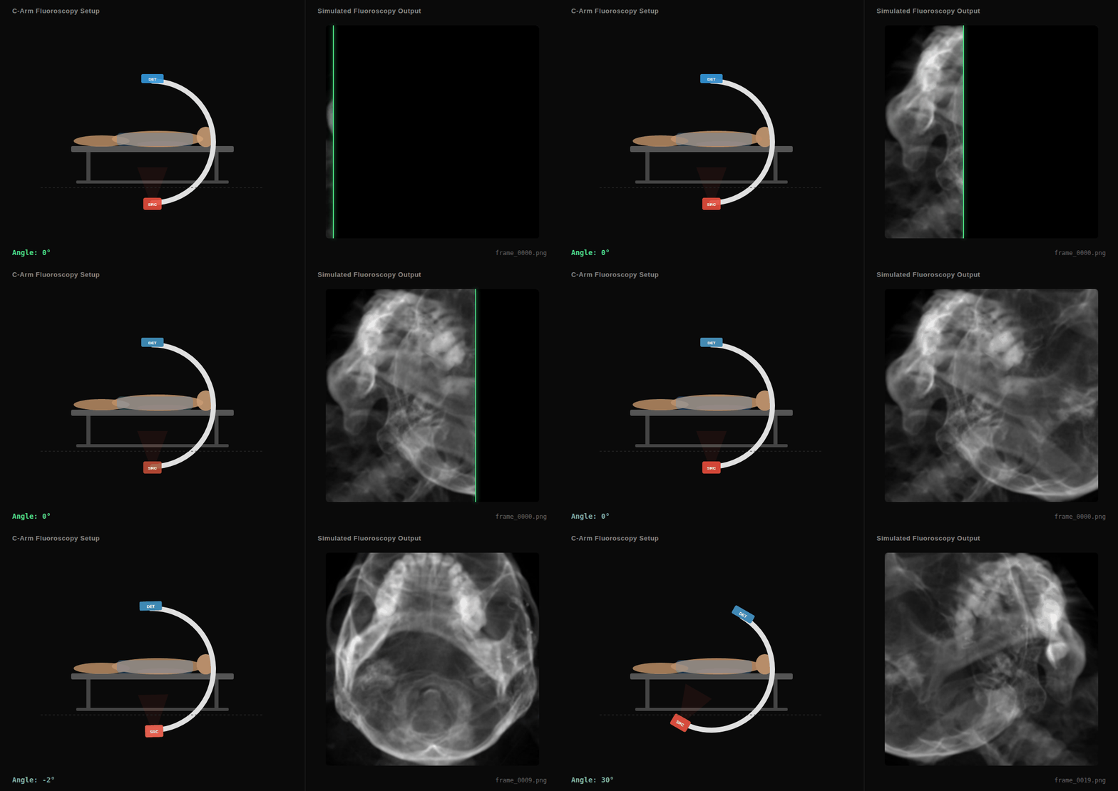
C-arm sweep animation showing the virtual X-ray source (SRC), detector (DET), and simulated fluoroscopy output in real-time.

---

Table of Contents

1. Installation
2. Quick Start
3. Architecture, API & Configuration — rendering pipeline, physics, API reference, C-arm configuration
4. Examples & Test Data — test datasets, example scripts, running the examples

---

Installation

Option 1: Using the I4H CLI (Recommended)

The ./i4h CLI builds and runs inside a Docker container with all dependencies pre-installed. Each step is a separate mode; the cached preprocessed volume persists between runs in xray-simulator/output/.

# Synthetic data workflow (no real CT data needed)
./i4h run xray-simulator preprocess_synthetic
./i4h run xray-simulator demo

# Real CT data workflow
./i4h run xray-simulator download_data
./i4h run xray-simulator preprocess_dicom
./i4h run xray-simulator demo

# List available modes
./i4h modes xray-simulator

# Launch an interactive shell inside the container
./i4h run-container xray-simulator

Set xray_simulator_OUTPUT_DIR or xray_simulator_CACHE_DIR to override the default output paths.

Option 2: Docker

cd xray-simulator

# Build the Docker image
docker build -t xray_simulator  .

# Run the container
docker run -it --rm --gpus all xray_simulator bash

# Inside the container
# Run the synthetic demo
python examples/preprocess_ct.py --synthetic
python examples/xray_simulator_demo.py

# Run the demo with real CT data
# Download the dataset
kaggle datasets download -d adamhuan/multiphase-ct-anigography-2-datasets
unzip multiphase-ct-anigography-2-datasets.zip
python examples/preprocess_ct.py --dicom excellent/excellent/0
python examples/xray_simulator_demo.py

Option 3: Bare Metal Installation

cd xray-simulator
pip install -e .[all]

Requirements:

Dependency	Purpose
CUDA-capable GPU	GPU-accelerated rendering
slangpy >= 0.40	Slang shader compilation and autodiff
numpy	Array operations
SimpleITK	DICOM/NIfTI loading (optional)
torch	PyTorch integration for autograd (optional)

---

Quick Start

from xray_simulator import VolumePreprocessor, xray_simulator, SimulatorConfig, PreprocessedVolume

# Step 1: Preprocess CT volume (HU → μ conversion)
volume = VolumePreprocessor.from_nifti("ct.nii.gz").preprocess()

# Step 2: Create simulator and render
simulator = xray_simulator(volume)
frame = simulator.render_frame(rotation=(0, 0.5, 0))  # 0.5 rad Y rotation

# Step 3: Save result
frame.save("output.png")

Step-by-Step Explanation

Step 1: Volume Preprocessing

CT volumes store tissue density in Hounsfield Units (HU). The VolumePreprocessor converts these to linear attenuation coefficients (μ in mm⁻¹) using a linear mapping:

μ = μ_min + (HU - HU_min) / (HU_max - HU_min) × (μ_max - μ_min)

Default mapping: HU ∈ [-1000, 3000] → μ ∈ [0.0, 0.02] mm⁻¹

# Load from various sources
volume = VolumePreprocessor.from_dicom("/path/to/dicom/").preprocess()
volume = VolumePreprocessor.from_nifti("ct.nii.gz").preprocess()
volume = VolumePreprocessor.from_numpy(hu_array, spacing_zyx_mm=(1.0, 0.5, 0.5)).preprocess()

# Cache to disk for fast reloading
volume = preprocessor.preprocess(output_dir="/tmp/xray_cache")

# Reload cached volume
volume = PreprocessedVolume.load("/tmp/xray_cache")

Step 2: Simulator Initialization

The xray_simulator initializes the GPU rendering pipeline:

simulator = xray_simulator(volume, config=SimulatorConfig())

• uploads μ-volume to GPU as a 3D texture with trilinear interpolation
• compiles Slang shader with autodiff enabled
• configures virtual C-arm geometry (source, detector, isocenter)

Step 3: Frame Rendering

Render a single X-ray frame at a specified C-arm pose:

from xray_simulator import Pose

# Clinical views, by name or by C-arm angles
frame = simulator.render_frame(pose=Pose.ap())
frame = simulator.render_frame(pose=Pose.lateral("left"))
frame = simulator.render_frame(pose=Pose.from_clinical_angles(30.0, 20.0))  # LAO 30 / CRAN 20

# Or a raw pose, in the renderer's own frame
frame = simulator.render_frame(
    rotation=(rx, ry, rz),      # Euler angles in radians, ZXY convention
    translation=(tx, ty, tz),   # Isocenter offset in mm
)

The presets assume the volume is in the canonical patient frame (+X Left, +Y Posterior, +Z Superior), which is what the digital-twin preprocessing produces and records in metadata.anatomical_frame. All of them put the head at the top of the image; AP shows the patient's left on the viewer's right, and the laterals are named by the side the detector is on.

Raw Euler angles have no anatomical meaning on their own, and the identity pose is an axial projection rather than a radiographic view. See World Frame and Pose Convention for the axis and rotation conventions, and for how to aim the isocenter at a patient-space point.

Step 4: Image Appearance

Rendering yields intensity I = i0 · exp(-∫μ ds), and DisplaySettings decides how that becomes pixels. There are two modes, and they differ only in which way round the greys go:

Mode	Preset	Dense structures	Looks like
Fluoroscopy (default)	"fluoro"	dark on a bright background	a live cath-lab monitor
X-ray	"xray"	bright on a dark background	a diagnostic radiograph / DRR

from xray_simulator import Pose, SimulatorConfig, xray_simulator

# Fluoroscopy, the default
simulator = xray_simulator(volume, SimulatorConfig.for_appearance("fluoro"))

# X-ray images instead
simulator = xray_simulator(volume, SimulatorConfig.for_appearance("xray"))

simulator.calibrate_display()   # fit the log window to this patient, once

Both modes come off the same render, so you can switch whenever you like — including partway through a session, or after a frame has already been rendered:

simulator.set_polarity("xray")     # flip modes, keeping the calibrated window
simulator.set_appearance("fluoro") # or load a whole preset (replaces the window too)

# Or keep the intensity and produce both looks from one render
simulator = xray_simulator(volume, SimulatorConfig
                           .for_appearance("fluoro")
                           .with_output(keep_intensity=True))
frame = simulator.render_frame(pose=Pose.ap())
frame.save("fluoro.png")
frame.with_appearance("xray").save("xray.png")   # same photons, other polarity

Both modes map intensity logarithmically, like a real detector chain, using a mapping that is identical for every frame so brightness stays stable while the C-arm moves. Calibrating is worth the one extra frame: the useful attenuation range depends on patient size and μ scaling, so the default window is a compromise. calibrate_display() measures it once and then holds it fixed, which is what distinguishes it from per-frame normalization (scaling="per_frame"), where brightness follows whatever is in the field of view and cine sequences flicker.

"diagnostic" is accepted as a synonym for "xray", and "fluoro_contrast" is fluoroscopy over a narrower window for more soft-tissue and contrast separation. The old physics.normalize / physics.invert flags still work and warn; together they are the "legacy" preset. See Image Appearance for the full table.

Step 5: Output

# Access rendered image as numpy array
image = frame.image  # Shape: (H, W), dtype: float32, range: [0, 1]

# Save to disk
frame.save("output.png")  # 8-bit grayscale PNG
frame.save("output.npy")  # Full-precision numpy

Rendering Multiple Frames (Cine Sequence)

from xray_simulator import Pose

# Generate a LAO/RAO sweep animation
poses = [
    Pose.from_clinical_angles(primary_deg=angle)
    for angle in range(-30, 31, 2)  # RAO 30 through LAO 30 in 2° steps
]

cine = simulator.render_cine(poses, fps=15.0)
cine.save_all("/tmp/output", format="png")  # frame_0000.png, frame_0001.png, ...

# Access as numpy array
frames_array = cine.to_numpy()  # Shape: (N, H, W)

---

Further Reading

• Architecture, API & Configuration — Physics model, differentiable rendering, full API reference, and C-arm geometry configuration.
• Examples & Test Data — Recommended datasets (e.g. Kaggle), command-line examples, single-frame/cine/streaming code, and step-by-step instructions for preprocess_ct.py and xray_simulator_demo.py.